Usage

This example demonstrates how to set up and use the Explainer with a basic lightgbm model trained on the Breast Cancer dataset. Note that similar configurations can be applied to other models, Explainer is also compatible with xgboost and catboost.

For detailed information, please refer to the API Reference.

Setup Code

from lightgbm import LGBMClassifier
from sklearn.datasets import load_breast_cancer
from sklearn.model_selection import train_test_split

from treemind import Explainer
from treemind.plot import (
    feature_plot,
    interaction_plot,
    interaction_scatter_plot,
)

# Load the dataset
X, y = load_breast_cancer(return_X_y=True, as_frame=True)

# Train the model
model = LGBMClassifier(verbose=-1)
model.fit(X, y)

Once the model is trained, it is ready to be analyzed with the Explainer.

Initializing the Explainer

After training the model, initialize the Explainer by calling it with the model object:

explainer = Explainer()
explainer(model)

Counting Feature Appearances

The count_node function analyzes how often individual features or pairs of features appear in decision splits across the model’s trees. This analysis can help identify the most influential features or feature interactions in the model’s decision-making process.

To count individual feature appearances in splits:

explainer.count_node(order=1)

| column_index | count |
|--------------|-------|
| 21           | 1739  |
| 27           | 1469  |
| 22           | 1422  |
| 23           | 1323  |
| 1            | 1129  |

To count feature-pair interactions in splits:

explainer.count_node(order=2)

| column1_index | column2_index | count |
|---------------|---------------|-------|
| 21            | 22            | 927   |
| 21            | 23            | 876   |
| 21            | 27            | 852   |
| 1             | 27            | 792   |
| 23            | 27            | 734   |

Analyzing Specific Feature

The analyze_feature function calculates statistical metrics for a specific feature based on its split points across the model’s trees. This analysis helps in understanding the distribution and impact of a single feature across different split points.

To analyze a specific feature by its index (e.g., 21), use:

feature_df = explainer.analyze_feature(21)

| worst_texture_lb | worst_texture_ub |   value   |   std    |  count  |
|------------------|------------------|-----------|----------|---------|
| -inf             | 18.460           | 3.185128  | 8.479232 | 402.24  |
| 18.460           | 19.300           | 3.160656  | 8.519873 | 402.39  |
| 19.300           | 19.415           | 3.119814  | 8.489262 | 401.85  |
| 19.415           | 20.225           | 3.101601  | 8.490439 | 402.55  |
| 20.225           | 20.360           | 2.772929  | 8.711773 | 433.16  |

To visualize feature statistics calculated by analyze_feature using feature_plot:

feature_plot(feature_df)

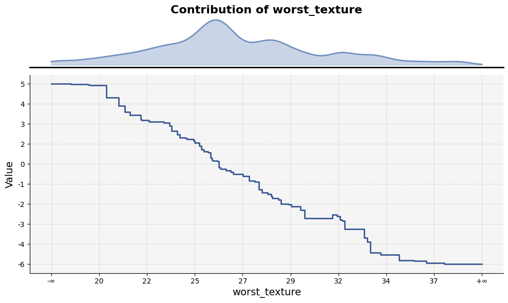
The feature_plot function plots the values of a specific feature based on split points across trees.

Analyzing Feature Interactions

The analyze_feature function given multiple indices calculates the dependency between two or more features by examining their split points across the model’s trees.

To analyze an interaction between two features (e.g., feature indices 21 and 22), use:

df = explainer.analyze_feature([21, 22])

Example output:

| worst_texture_lb | worst_texture_ub | worst_concave_points_lb | worst_concave_points_ub |   value   |   std    |  count  |
|------------------|------------------|-------------------------|-------------------------|-----------|----------|---------|
| -inf             | 18.46            | -inf                    | 0.058860                | 4.929324  | 7.679424 | 355.40  |
| -inf             | 18.46            | 0.058860                | 0.059630                | 4.928594  | 7.679772 | 355.34  |
| -inf             | 18.46            | 0.059630                | 0.065540                | 4.923128  | 7.679783 | 355.03  |
| -inf             | 18.46            | 0.065540                | 0.069320                | 4.912888  | 7.682064 | 354.70  |
| -inf             | 18.46            | 0.069320                | 0.069775                | 4.912888  | 7.682064 | 354.70  |

To visualize interactions between two features calculated by analyze_interaction using interaction_plot:

interaction_plot(df)

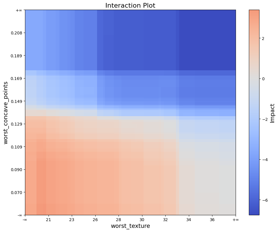
The interaction_plot function visualizes feature interactions by creating a filled rectangle plot. The plot uses model split points to display intervals, with color intensity representing the interaction values.

To visualize interactions between two features on given data by analyze_interaction using interaction_scatter_plot:

interaction_scatter_plot(X, df, 21, 22)

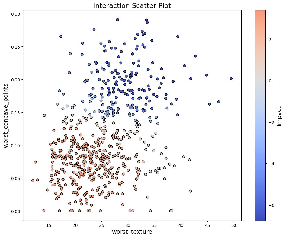
The interaction_scatter_plot function visualizes feature interactions reflected on given data.